[1] 2875 54Patient Satisfaction Predictions for Emergency Department Encounters Using Multivariate Regression

Abstract
Patient satisfaction can be an indication of quality care and aid in predicting health outcomes and patient retention. Although subjective, it is crucial for healthcare administrators to understand and meet patients’ expectations, translate it to patient-oriented care within delivery models, and improve population health as a result. The project requirement was to use a multivariate regression model, though a Poisson regression would have been more appropriate given the count-based nature of the response variable. This project investigates features associated with higher patient satisfaction scores for ER encounters and developing models to predict them.
Data
This data set is a patient satisfaction survey administered to patients discharged from ten different entities at NMH over the span of two years. Respondents were discharged from six emergency units. Surveys were delivered either on paper or electronically following their encounter. The patient satisfaction surveys collected, range from discharges starting March of 2016 through January of 2018. Responses were given in either English or Spanish. Five types of payers were used for the encounters and satisfaction scores per response were given on a scale of one (very dissatisfied) to five (very satisfied). No other information on how the data was collected is available.
Population of Interest
The population of interest is the patient population for emergency encounters at NM with disproportionately lower social determinants of health.
Exclusion Criteria
A waterfall approach was used to define the population of interest. Social determinants, which include environmental and non-health related factors such as socio-economic status, can account for 30-55% of health outcomes1. Payer type was used as a proxy to define subsets of the population with disproportionate social determinants, with financial payers like Medicaid typically insuring low-income individuals. Self-pay and Medicaid payers were also included in the drop-down conditions, as this subset tends to misuse the ER for non-urgent care, serving as a viable proxy for lower health literacy.2. Patterns of ER misuse are also more likely to be younger and of non-hispanic black race, however, the only information available an race were responses indicating white or non-white. While sub-setting race to only non-whites would align more with the population of interest, this information was retained to maintain the basis of interpretation and prevent over specification of models in the event covariates are used. The age at which we thought individuals could best understand and articulate aspects of the emergency department setting was 16 years old. Records younger than that were omitted.
After cleaning records and additional formatting, observations were then cleaned. Survey ID 1418129390 had missing admit and discharge times and the encounter record for the survey was dated 1900-01-01. The implicit erroneous record was removed.
To maintain the integrity of the data set, observations with missing discharge or admit times were removed.
Observations were subset to those over the age of 16 who were Medicare, Medicaid, or Self-Pay users to isolate the patient population. No demographic attributes were missing thereafter.
Respondents were asked to survey their satisfaction across different care settings during their encounter. The Likert scale of possible responses were 1-5.
For the non-demographic survey questions, there were a number of missing responses. Survey respondents that had greater than 30% of answers missing were removed from the drop down conditions. Subsequently, survey questions across the sample that had more than 30% of responses missing were also omitted. The questions removed were:
A87 (Arrival) - Helpfulness of person who first asked you about your condition D2 (Tests) - Courtesy of the person who took your blood D52 (Tests) - Concern shown for your comfort when your blood was drawn
A new variable was created to measure the length of time between discharge date and the date the survey was received. Survey IDs with negative response times were present, implying that they received the survey before being admitted to the ER. These records were concluded as an error and were also omitted.
Survey responses could be grouped into one of the following care setting categories: Arrival, Personal/Insurance Info, Nurses, Doctors, Tests, Family or Friends, Personal Issues.
For any missing responses afterwards, the missing values were replaced with the average satisfaction score for that question.
Model Validation Setup
[1] 2049 55[1] 826 55Methods
A regression model was fit to predict the overall patient satisfaction variable, F68, and used to estimate the true population parameters. A 70/30 train:test ratio was used for model validation. Regression assumptions were then validated. For residual normality and increased model accuracy, explanatory variables were transformed before model fitting. The sampling distribution forms a left-skew distribution, in which the sixth root and natural log transformations were applied.
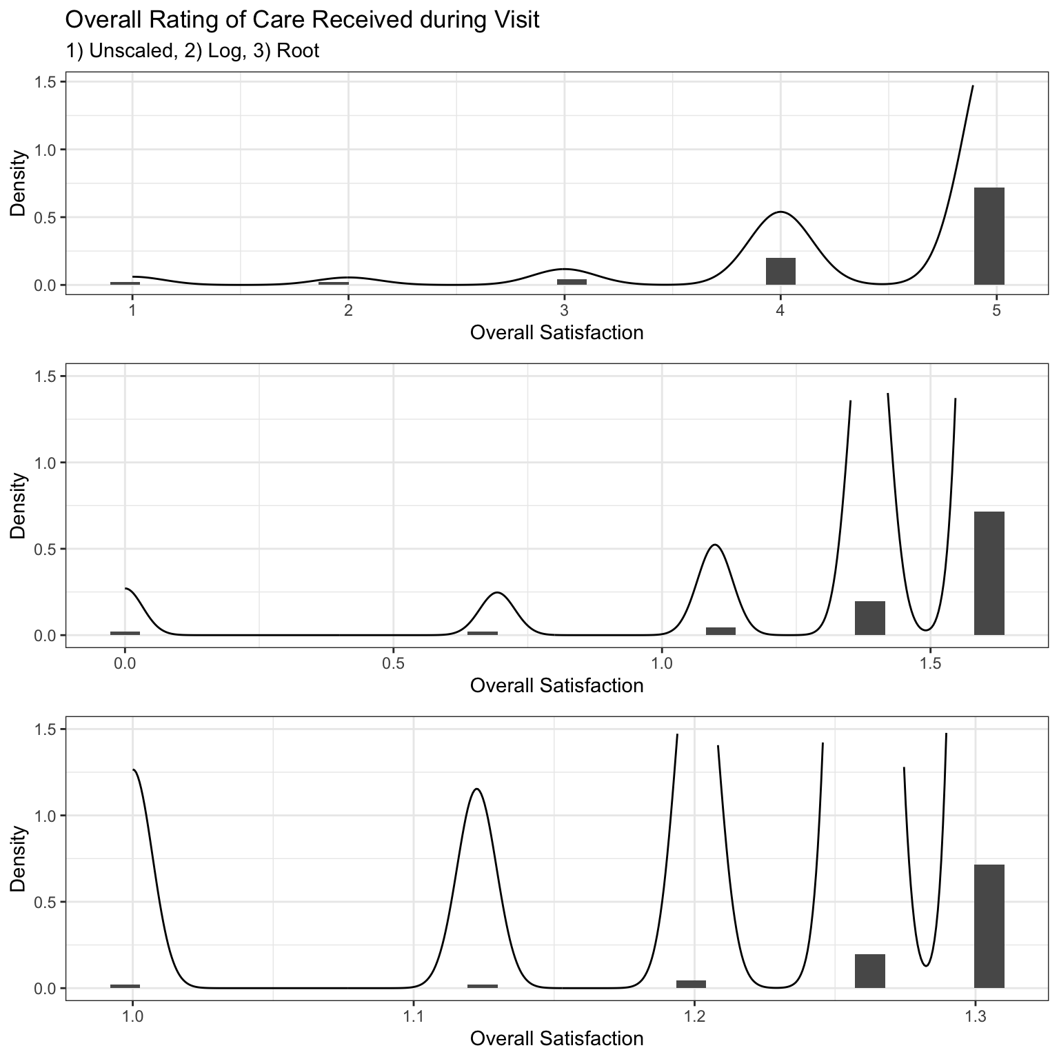
Observing that the root transformation resulted in the greatest shift towards normality, it was applied to all explanatory variables. Additionally, summary variables based on category were calculated to enhance predictive power, specifically by computing the mean averages for each category. Several transformations were performed on the predictor variable F68 to improve the overall coefficient of determination and model fit. Consequently, the final explanatory parameters are based on the root of F68.
Pearson’s product correlation matrix was used for variable selection; starting with the highest coefficient of determination, a regression model was fit in progressive steps with one or two variables at a time. At each step, a combination of diagnostic tests and empirical thresholds were used to assess goodness-of-fit based on the following criteria:
\[ Δ R^2 = R_f^2 - R_n^2 > .2 \]
Where the additional variable must increase the coefficient of determination by 2% in order for the variable to be retained.
Turkey’s Nonadditive Test was used to asses presence of interaction. In the context of regression, fitted values squared are computed post-hoc as a quadratic function to test if the interaction term is significantly different from zero, assuming H0: ŷ = 0 and a linear function is modeled with Ha: ŷ ≠ 0 and a non-linear function is modeled:
\[\hat{f_n} = (β_1)\hat{x_1} + (β_2)\hat{x_2}+ (β_3)\hat{x_3}...+(\hat{y_n})^2\hat{x_z}\]
\[\hat{y_n} = (β_1)\hat{x_1} + (β_2)\hat{x_2}...+(β_z)\hat{x_z}\]
where ŷf are the full predicted values and ŷn are the nested predicted values, variables were retained if P(F) < .05.
Difference in fits was used to measure the influence of individual observations obtained using an empirical threshold of \({\small √(p)/n}\); where p is the number of parameters and n is the number of observations
Cook’s distance uses leverage and studentized residuals to measure significance of observation on overall model; threshold of 4/n was considered to be practically influential and was further evaluated
Wald Statistic: {\(β^2/Var(β)\)} measures the effect size of individual parameters.
Variance Inflation Factors greater than four were reevaluated; greater than seven are removed.
The model yielding the optimal Δ R2 and least RMSE was used as the production model. The questions used to guide the final model were:
- Does the model capture the true population parameters and relationship? Can the model be used to draw generalizations from our target population?
- Is the model an accurate predictor of patient satisfaction?
The results of the diagnostic post-hoc tests were then used to assess the models capability to generalize to the target population and decide if a different model would be more equipped to capture the relationships found in survey responses to overall patient satisfaction in ER encounters for those with low social determinants of health. In practice, it is acknowledged that no generalizations can accurately be made on our target population due to the limited information around how the data was collected. It is unknown if the observations were from a random sample, which is sufficient and necessary to make any population conclusions. Any aforementioned hypothesis to the population is for the sake of statistical inference and this endeavor. However, to validate prediction capabilities, a precision grade was used on our test set.
Analysis
Pearson’s product correlation plot showed that overall satisfaction was strongly correlated with how well patients were informed about delays and other responses based on either doctors’ or nurses’ care setting.
| Variable | Correlation | Category | Question |
|---|---|---|---|
| F2 | 0.796 | Personal Issues | How well you were kept informed about delays |
| B3 | 0.734 | Nurses | Nurses’ attention to your needs |
| B4 | 0.733 | Nurses | Nurses’ concern to keep you informed about your treatment |
| C4 | 0.727 | Nurses | Doctor’s concern for your comfort while treating you |
| C2 | 0.674 | Doctors | Courtesy of the doctor |
| B5 | 0.655 | Doctors | Nurses’ concern for your privacy |
| C1 | 0.629 | Doctors | Waiting time in the treatment area, before you were seen by a doctor |
F2 was therefore used as the initial predictive variable and subsequent variables were added in a ‘stepwise’ fashion while assessing the change in R2 and MSE. Variables within the same category exhibited a high degree of underlying collinearity and summary statistics were calculated for the means of the top two responses or the total responses per group to remediate covariance. This is preferable since 1) information can be easily summarized into one parameter instead of multiple, decreasing the Alkaline Information Criterion while maintaining parsimony and 2) missing responses are a notable characteristic of survey data and limiting the model to individual parameters can lead to inaccuracy for future data sets that have large proportions of missing responses to individual questions.
Results
The final regression is modeled by
\[ f(x) = -3.52083 + 1.94361*x_1 + 1.35390*x_2 + 1.11454*x_3 \] \[ RMSE = .12 \]
where β1 describes change in ŷ for a one unit change in the root mean satisfaction for the personal issues category, β2 for a one unit change in the root mean satisfaction for the nurses category, and β3 for a one unit change in the root indicator for Doctor’s concern for patients comfort while treating them. Interpretations for β0 is omitted due to transformations and range of the data set. The Adjusted R2 ~ .74, F(3,2045), p = 2.2e-16 using adjusted Type I error rate = .005.
Our model produced a MSE = 0.015 (RMSE = 0.123) with statistically significant results for all predictors. The RMSE quantifies the models predictive capability in the context of regression such that it measures the average difference between the observed values and the predicted values of our model. In other words, the model predicts overall satisfaction within .12 of the actual satisfaction scores for the training data set. Although robust and promising, true confirmation of performance is assessed on the training data set via precision grades below.
Analysis of Variance Table

Response: F68_rt
                       Df Sum Sq Mean Sq F value    Pr(>F)
personal_issues_3_rt    1 76.254  76.254 5196.77 < 2.2e-16 ***
nurses_3                1  5.688   5.688  387.64 < 2.2e-16 ***
C4_rt                   1  3.280   3.280  223.52 < 2.2e-16 ***
Residuals            2045 30.007   0.015
---
Signif. codes:  0 '***' 0.001 '**' 0.01 '*' 0.05 '.' 0.1 ' ' 1
If the data was obtained via random sampling, the model then could be used as an estimate for the true target population’s overall satisfaction. Residual plots were used to test residual normality and linearity with P(F) = .57 on one degree of freedom for Tukey’s test for non-additivity. Residual values lie within three standard deviations with a few minor exceptions in the fitted values, prompting an opportunity for different optimization methods. The apparent uncaptured variation between the predictor variables calls for models suited for continuous ordinal data such as logistic, poisson, or generalized linear models that can capture different types of distributions.
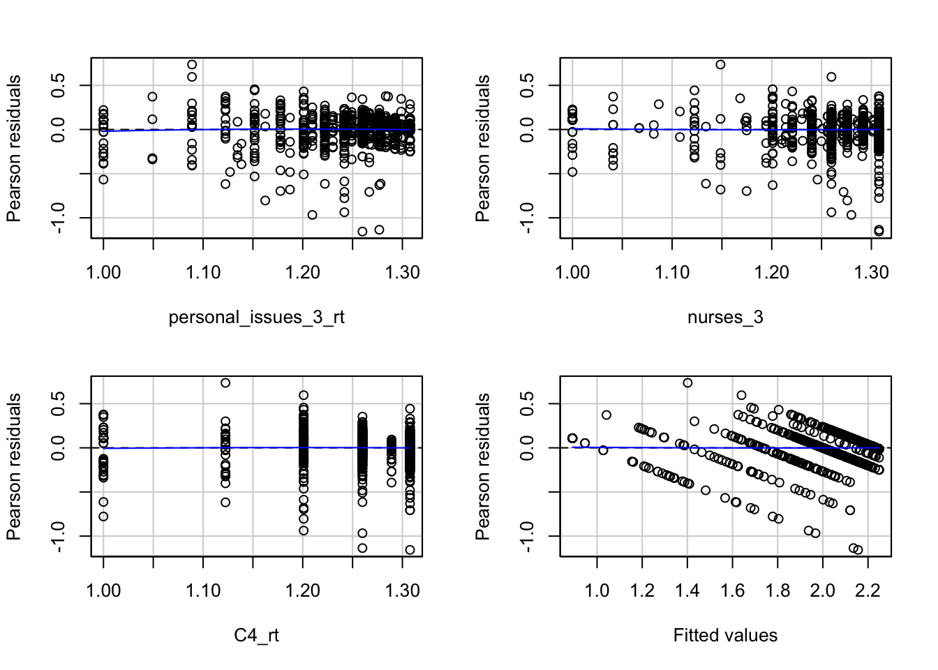
                     Test stat Pr(>|Test stat|)
personal_issues_3_rt   -1.3799           0.1678
nurses_3                0.6213           0.5345
C4_rt                  -0.5763           0.5645
Tukey test              0.3667           0.7138
Survey IDs 1344260683 and 1439794901 had the highest influence on the overall model in comparison to the global average of Cook’s distance. Looking at the original data, the former had missing responses for four of the seven questions used to produce the model, highlighting a major flaw in this model - its predictive inaccuracy for patients with missing responses - as missing responses were filled with grand means after exclusion criteria were applied. Although missing at random, a better approach would be to fill in with median values or apply more conservative exclusion factors such as omitting observations with greater than 10% of responses missing. The latter was greatly considered, but the trade-off of small sample sizes and subsequent over fitting were outweighed.
After confirming the absence of variance inflation, the Log Likelihood ratio test was done for the nested model excluding x3, as this was the only non-summary predictor. Wald statistics are limited for linear models such that P(Wald) > P(LRT). Assuming null hypothesis is true where the nested model is just as adequate as the full model, p(χ) = 1.2e-48 (215,1) the affect of x3 on the model is statistically significant.
'log Lik.' 214.9064 (df=4)[1] 1.168115e-48Model Validation
The challenge with model validation is being conscious of the present data and methods taken throughout the modeling process on the test set and appropriately applying them chronologically on the test set. Inefficient processes/workflows used in the modeling phase will often reveal itself in testing. The variance-bias tradeoff is the central phenomena that typically only be visualized during testing. While there are preventative measures analysts take initially to prevent this such as model specification and applied weights, benchmarks need to be created to measure the ability to be precise and to maintain that precision on unseen data.
After using the parameters from the trained model to calculate the predicted satisfaction scores of our test set, the Mean Absolute Error (MAE) was used to calculate percent accuracy for the test. Arbitrary cutoff points where then assigned four grades ranging from letters A through F- given the following criteria:
Variance/Bias Tradeoff
The grades are only one of many test diagnostics used to measure how well a given model fits a subset of data (model fit) and how well it fits unseen data. The risk in the former is fitting a model too well. There are two common scenarios that both are operational and are forms overfitting and underfitting. The first being that the trained model fits very well on the initial data. These models will exhibit properties that are ‘too good to be true’ such as an RMSE ~ 0 or a predictive accuracy ~100%. The issue then becomes a lack of flexibility - mainly components of lack of parsimony, very few observations, or unrecognized bias in data (not to be confused with modeling bias). These models often perform very poorly on new data. With regard to the latter, underfitting is less common and exhibits the converse process. Upon initial assessment, the grades look promising. The absolute value of the difference between the predicted and observed values are reported as proportions and easier to interpret below. The model predicted satisfaction score for each patient is within 91% of the actual score. 1.9% of patient satisfaction scores were off by greater than 25% on the polar opposite (F -). Visualizing the models outputs reveals the ostensible performance of the model.
| forward.PredictionGrade | Freq |
|---|---|
| Grade A: [0,0.10] | 0.9176755 |
| Grade B: (0.10,0.15] | 0.0375303 |
| Grade C: (0.15,0.25] | 0.0254237 |
| Grade F-: (0.25+] | 0.0193705 |
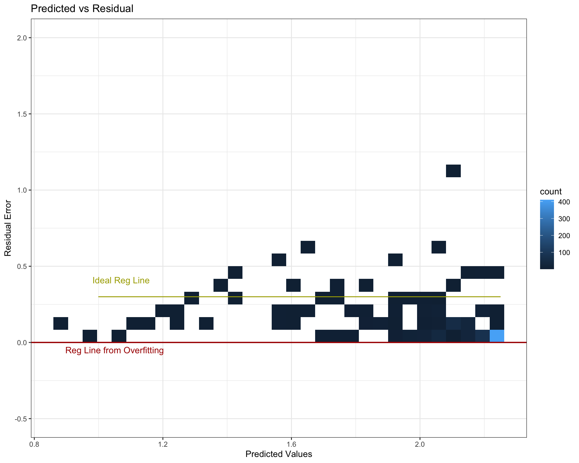
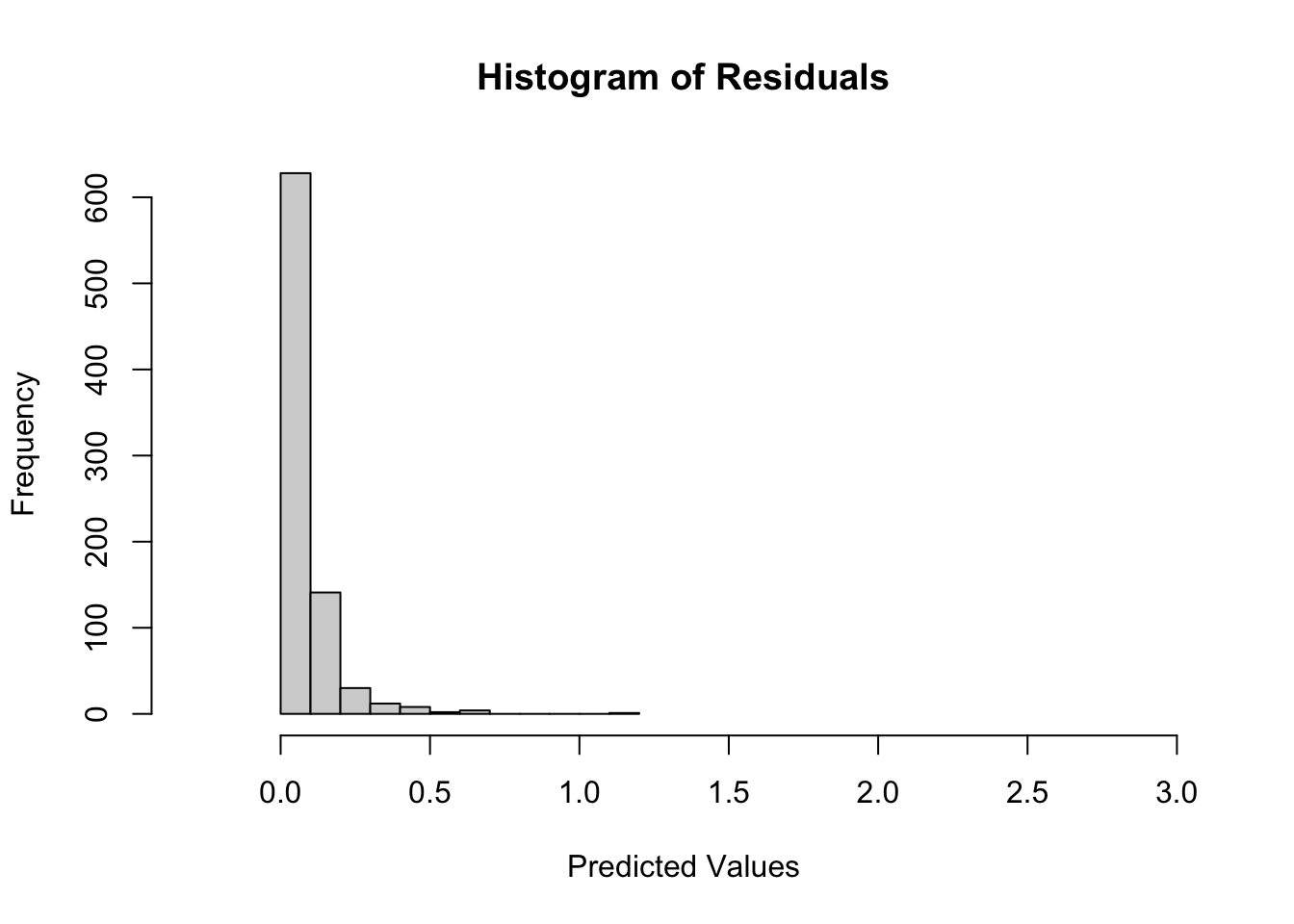
Predicted vs Residuals
The first plot is a density bin plot where the x axis are the predicted values and the y axis are the residuals or how much the model was off by. Note that these units are not to scale with the original patient satisfaction scores since the data was transformed for model compatibility. The red line indicates where the error (and data) should be centered. Robust models, and the goal of optimization in the OLS regression, is to fit a line on a cloud of data such that the residual error is zero (if predicted and actual values are the same, the model is 100% accurate and residuals equal zero). This is idealistic and impractical, but nevertheless is what’s being optimized. The red line sits beneath all data points, indicative of severe over fitting. For all patients, the model over predicts patient satisfaction and most likely will for future data sets. The fully optimized estimated regression line most likely runs somewhere where the yellow line is. Not only would the model be more balanced in regard to variance-bias, residual normality is the underlying assumption for OLS normality.
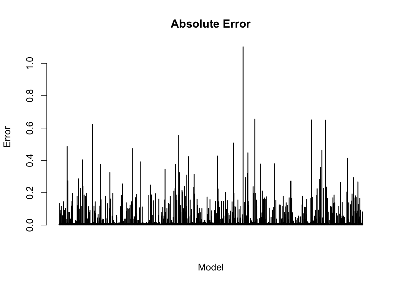
Absolute Error
The produced residuals from testing form a right skew log-normal distribution. During wrangling, the sampling distribution had an identical distribution but was skewed left. The severe deviations from a centered distribution with relatively even kurtosis may result in long-term predictive inaccuracies if not remedied. The last visualization shares similarities with influence visualizations. The x-axis is indexed to the error on the y-axis, allowing for comparisons of individual residual errors for each observation across the test data set. The indexes with taller heights can be an implication of the observations individual impact to the model. Models with balanced variance-bias should have uniform height.
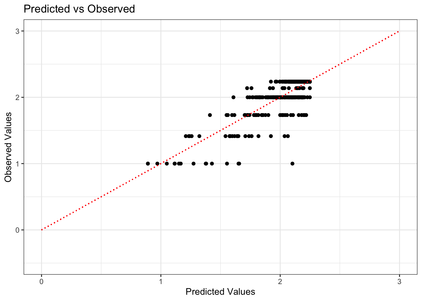
Predicted vs Observed
Residual values against predictions can reveal the presence of normality. If the model performs at a 100% accuracy, the predicted and observed values should be 1:1 and the points should subsequently form a regression line with as close to a slope of one as possible. Granted, this is more difficult to accomplish given the nature of the data set. Patient satisfaction scores are discrete values that take whole numbers from 1-5 in the original data set, the reason there are ~5 discrete lines that are shown below.
Conclusion
The ability to quantify and understand the relationships between different hospital staff interactions during emergency care encounters can be powerful for creating quality and retention initiatives within communities with lower social determinants of health. The model revealed that key predictors of overall patient satisfaction included the doctor’s attention to the patient’s care, communication about delays, the degree to which staff demonstrated care for the patient as an individual, how well pain was controlled, and the attention and courtesy provided by nurses. By focusing on these critical aspects of care, especially in patient populations like Medicaid, Medicare, and self-pay patients, hospitals can implement targeted quality improvement initiatives that address the specific needs of these groups. Enhancing these areas not only improves patient satisfaction but also promotes better retention and long-term health outcomes. This data-driven approach enables healthcare providers to offer more personalized, effective care, ultimately fostering a more equitable and satisfying patient experience in communities with significant social and economic challenges.
Footnotes
Williams JN, Drenkard C, Lim SS. The impact of social determinants of health on the presentation, management and outcomes of systemic lupus erythematosus. Rheumatology (Oxford). 2023 Mar 29;62(Suppl 1):i10-i14. doi: 10.1093/rheumatology/keac613. PMID: 36987604; PMCID: PMC10050938.↩︎
Naouri D, Ranchon G, Vuagnat A, Schmidt J, El Khoury C, Yordanov Y; French Society of Emergency Medicine. Factors associated with inappropriate use of emergency departments: findings from a cross-sectional national study in France. BMJ Qual Saf. 2020 Jun;29(6):449-464. doi: 10.1136/bmjqs-2019-009396. Epub 2019 Oct 30. PMID: 31666304; PMCID: PMC7323738.↩︎